Examples
Animated comparisons of pyakima against SciPy’s cubic splines. The images
follow the light/dark toggle in the sidebar.
Corner models
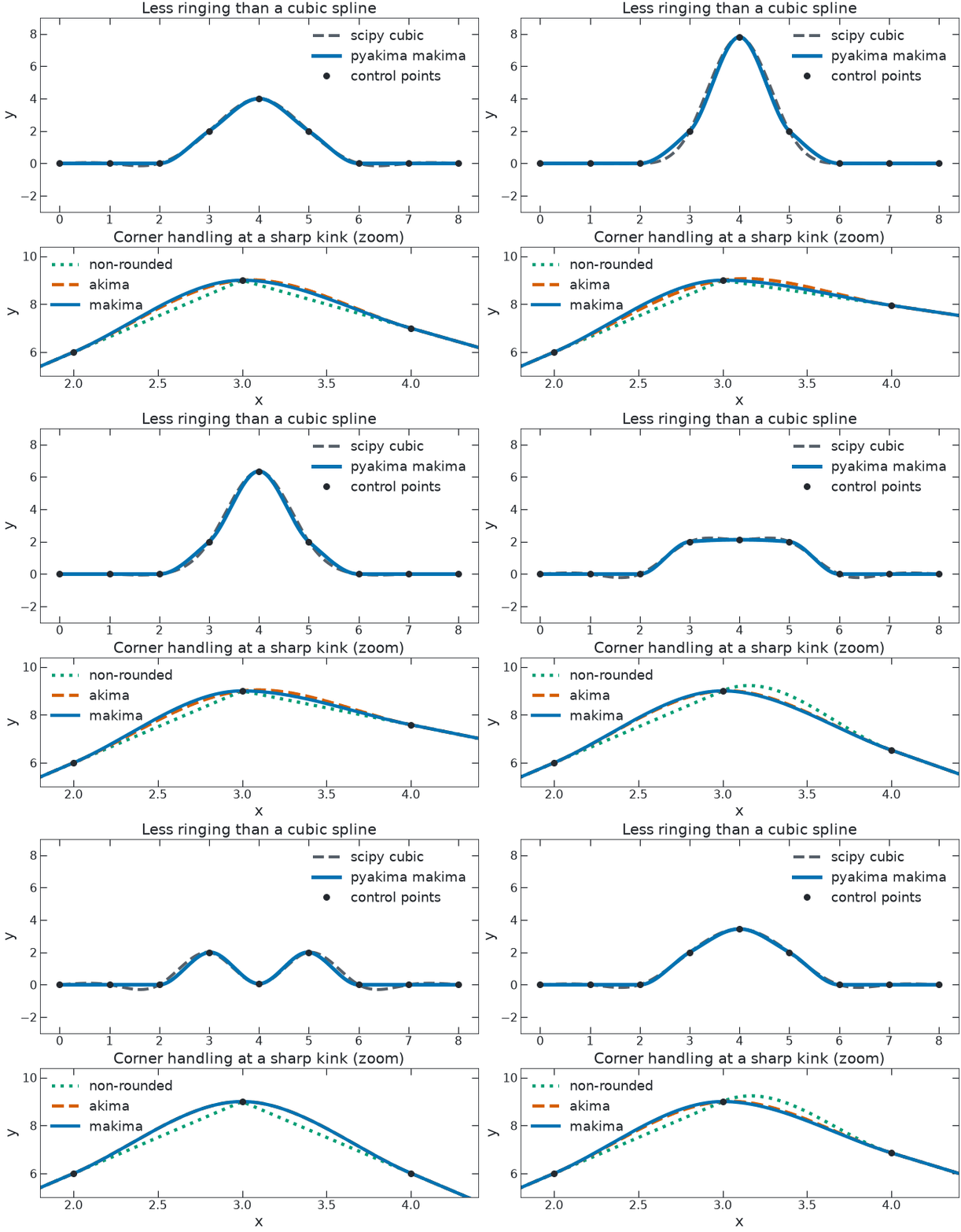
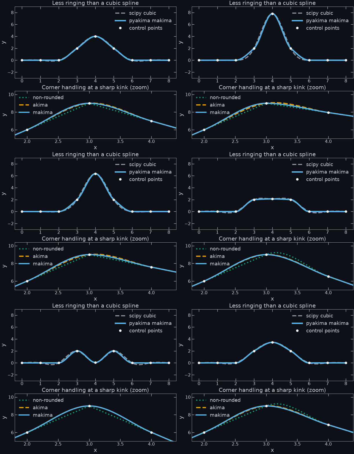
The top panel slides one control point up and down: the pyakima makima fit
stays local and flat on either side of the spike, while a natural cubic spline
rings above and below it. The bottom panel zooms into a sharp kink to show the
three corner models pyakima exports:
non-rounded: Algorithm based on [1], comparable numerical behavior to GSL; note the unstable behavior is because the algorithm is non-differentiable at corners, not a peculiar limitation of this implementation [2].akima(SciPy parity) [3]. Discontinuous behavior is less severe thannon-rounded; slightly more prone to overshoot, and still has special edge-case handling.makimaModified Akima Algorithm [4]; recommended default Less overshoot thanakima, while mathematically guaranteed to preserve differentiability/continuous behavior at corners without special edge-case handling. Similar performance toakimain most cases.
Irregular grids
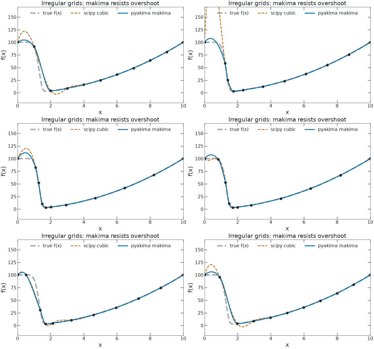
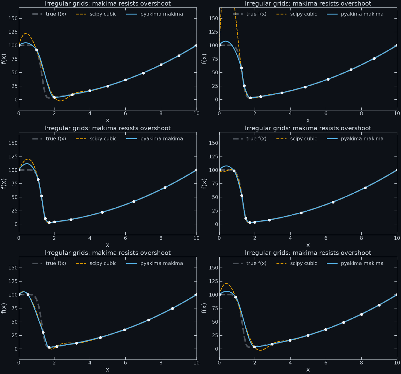
The control points oscillate smoothly between regular uniform-grid spacing and an inverse-CDF-based spacing.
Such a spacing is similar to what might be used when using Akima splines for a PSD estimation task, or in approximating a function
with sharp features with as few control points as possible. Such uses with irregular grids are a key modern application of Akima splines,
and are of central importance to their utility in gravitational-wave detection applications, such as using trans-dimensional MCMC
to adaptively fit Akima splines to un-modeled gravitational-wave sources [5], [6], [7].
Cubic splines, such as scipy’s default CubicSpline plotted above, oscillate wildly on the same irregularly-spaced grid, which typically makes them unsuitable for such analysis tasks.
Regenerating the Demo
pyakima.demos ships as an example subpackage; run it from a source checkout so
it can write the README assets:
pip install -e '.[demos]'                  # scipy, matplotlib, pygsl_lite
python -m pyakima.demos.animate_demo       # writes assets/akima_demo_{light,dark}.gif
python -m pyakima.demos.animate_grid_demo  # writes assets/akima_grid_{light,dark}.gif
python -m pyakima.demos.step_demo          # writes assets/akima_step_{light,dark}.png
References
G. Engeln-Müllges & F. Uhlig, Numerical Algorithms with C, Springer, 1996, ch. 13 “Akima and Renner Subsplines,” Algorithm 13.1. ISBN 978-3-642-64682-9.
Note: the internals of the GSL implementation have never been viewed by the repository author. However, calls to GSL exhibit near-identical behavior, supporting that the issue is algorithmic rather than due to implementation error.
Akima, Hiroshi. “A new method of interpolation and smooth curve fitting based on local procedures.” Journal of the ACM (JACM) , 17.4, 1970, pp. 589–602.
C. Moler, Makima Piecewise Cubic Interpolation, Cleve’s Corner (MathWorks blog), 2019.
Detecting gravitational wave signals using a flexible model for the amplitude and frequency evolution. T Gupta, NJ Cornish. Physical Review D, 2024•APS arXiv:2404.11719.
Model-agnostic gravitational-wave background characterization algorithm. T Knapp, PM Meyers, AI Renzini.Physical Review D, 2025•APS. arXiv:2507.08095
“Precise analysis of gravitational waves from binary neutron star coalescence using Hilbert–Huang transform based on Akima spline interpolation.” Yoda, Itsuki et al. Progress of Theoretical and Experimental Physics (2023). DOI:10.1093/ptep/ptad101